Mathcad Community Challenge March 2026: The Two Body Problem

The challenge

This month’s challenge was inspired by one of the great unsolvable challenges of physics, the Three Body Problem. To make it solvable, we challenged people to address the Two Body Problem for orbital mechanics:

Challenge 1: Create the math functions and programs that can calculate the position, velocity, and acceleration of a Mazda Miata-sized satellite in orbit around the earth. (Why a Mazda Miata? It was my first and only car. Feel free to substitute a car of your choice.)
Choose your orbital parameters for altitude (e.g., medium-earth, geosynchronous, high-earth), inclination, eccentricity, and any other factors.
Challenge 2 (optional): Incorporate advanced input controls to change the orbital parameters.
Challenge 3: Graph the x-, y-, and z-values for acceleration versus time. Create additional graphs for velocity and position. Bonus points for using the Chart Component.
Challenge 4: Create a 3D plot of the orbit of the satellite around the earth.
Challenge 5 (optional solvable Three Body Problem variant): Take on any special case or simplified version of the Three-Body Problem. For example, use a system consisting of the sun, earth, and Miata; or a sun-earth-Miata system with circular orbits; or a Lagrange Equilateral Triangle.

My take

I think this may be one of the hardest challenges we have had. The Three-Body Problem has vexed physicists and mathematicians for literally over 3 centuries. Having worked at Blue Origin, I know how complex orbital mechanics are. Even with only two bodies, this challenge involves complex functions and programs with differential equations. I am not surprised there were few takers.

The submissions

Frequent contributors Alan Stevens and Professor Tokoro both submitted worksheets.
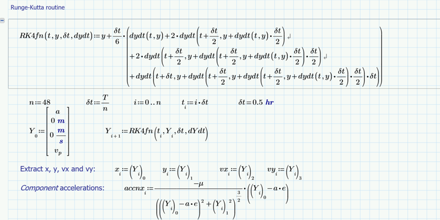
I always like the worksheets that Alan Stevens submits because I can understand them and his logic easily. He walks through setting up the equations of motion and orbit in a straightforward manner and then, wow, manually defines a 4th order Runge-Kutta function. He passes initial conditions to the functions and computes the accelerations in x, y, and z. He then uses XY Plots to graph the acceleration, velocity, and position. This is a great worksheet for aerospace engineering students.

How PTC solutions are used in aerospace

Aerospace enterprises and their partners deploy PTC solutions to address their challenges.

Learn More

It should be noted that Alan does all his work in the Mathcad Express version. That means he has to figure out these problems with less functionality, but it also makes his work accessible to a wider population.

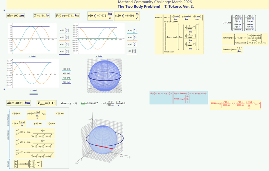
The first worksheet submitted by Professor Tokoro is a compact 2 pages. (There are several reused plotting functions hidden in a collapsed area.) It starts with Python code generated by Microsoft Copilot. Normally, I would shun the use of AI. But we are talking about the Three Body Problem; I considered using AI myself. Professor Tokoro translated the Python code into Mathcad Prime. He then plotted the components of acceleration, velocity, and position versus time with XY Plots. The earth and satellite orbit were then displayed in 3D Plots.

Version 2 was a single page, with all the math hidden in collapsed areas or the draft view. This version adds Combo Box basic input controls where users can change the altitude and velocity. A Solve Block calls a differential equation solver, and the results are updated in a 3D Plot.

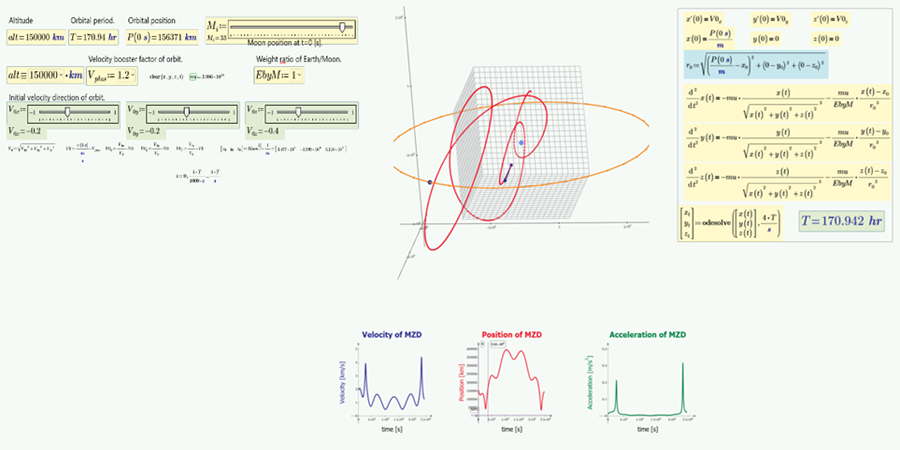
Version 3 adds even more advanced input controls; this time, slider controls allow you to alter initial velocity directions. Altering the values really conveys how small changes have huge effects on orbital stability. Version 4 fixed an error in version 3 regarding the crash point on the Earth for an unstable trajectory. However, this was submitted right after PTC Community returned from a hiatus; all we have is a PDF, so it’s not possible to investigate the worksheet changes or vary the orbital parameters.

Professor Tokoro’s fifth worksheet is very cool and should be viewed by all aerospace engineers. Instead of examining a two body problem with the Earth and a human-made satellite, it’s the Earth and its natural satellite – the Moon! I like how you can toggle between an Earth – Moon mass ratio of 80 and 1. In addition to varying the initial velocity directions, you can change the altitude, a velocity booster factor, and Moon position. With equal masses, you really can visualize how unstable the system is.

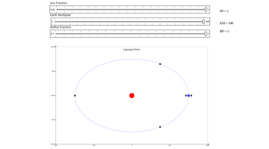
So that there was something addressing the solvable variants of the Three Body Problem, I submitted a worksheet for the restricted case of circular orbits involving the Sun, Earth, and an object of relatively insignificant mass. Although I had watched a few YouTube videos, I figured it would take some time to figure out Mathcad Prime’s Runge-Kutta differential equation solvers. I went the easy route and calculated the 5 semi-stable Lagrange positions using known equations and Mathcad Prime’s Solve Blocks (my favorite functionality). I added slider controls so people could see the effect of varying mass and orbital radius.

What can we learn?

Even a Two Body Problem or a restricted Three Body Problem can be quite a challenge to solve with numerical methods and differential equations. But Mathcad Prime – and Mathcad Express – contain the tools to compute orbits and trajectories. We can convey the results in 2D and 3D. The input controls in Mathcad Prime provide a deeper understanding of the complexity of these problems by allowing us to see the effects of changes immediately.

If Mathcad Prime can address these centuries-old problems, how can you apply it in your engineering problem solving and product development?

Join us in May for a geometry-based challenge inspired by the greatest rock band of all time!