Mathcad Community Challenge July 2026: Tautochrone & Isochronous Curves

The challenge

The July 2026 challenge was about tautochrone curves and isochronous curves. They involve placing an object on the curve and allowing it to slide without friction. With a tautochrone, an object placed at any point on the curve will take the same time to slide to the bottom. With isochronous curves, objects allowed to slide from any part of the curve will have the same period of oscillation. You can think of the tautochrone as “half” of the isochronous curve.
The challenge was as follows:

Challenge 1: Derive the equation of the tautochrone or isochronous curve.
Challenge 2: Graph the curve on an XY Plot or in the Chart Component.
Challenge 3: Find a function for the velocity of the object at the bottom based on either the starting height of the object, the starting horizontal distance, or the distance along the curve.
Challenge 4: Graph the results of Challenge 3.
Challenge 5: Calculate the period of oscillation in this scenario for the isochronous curve.
Challenge 6: How does the equation for the tautochrone / isochronous curve compare to the brachistochrone curve?

Brachistochrone curve explained (with some help from Mathcad)

Read how Dave Martin once used PTC Mathcad Prime’s tools to investigate the brachistochrone.

Read Dave’s Previous Work

The submissions

We had two great submissions this month, from Alan Stevens and Larry Julyk. We can declare Alan Stevens the winner of this challenge, as he addressed all six proposed challenges.

Larry Julyk’s worksheet derived the equations of motion for the related brachistochrone curve in a very cool way. I see the challenges as a starting point. If someone wants to take the idea and run in a different direction, I fully encourage that.

Alan Stevens’s Worksheet

I love, love, love this worksheet.
This has so many of the elements that make a worksheet a pleasure to read: organization, documentation, logic and derivation explained with the Comparison Equals To operator, visual presentation of results, and conclusions that are presented clearly in a document that can stand on its own as a teaching aide.
Challenge 1 derives the equation for the curves using the Lagrangian and the Euler-Lagrange equation. It uses derivatives, partial derivatives, double prime operators, integrals, and symbolic evaluation. The result from symbolic evaluation was messy, as Alan described it, so he based the rest of the challenge on a function involving a definite integral.
In challenge 2, Alan graphs the isochronous curve on an XY Plot using parametric equations from challenge 1, while also calculating the period (which satisfies challenge 5). Challenge 3 equates kinetic energy with potential energy for the velocity at the bottom, and that velocity is plotted in challenge 4 as a function of the starting distance along the curve. (Since the period / time to traverse has to be the same regardless of starting position, an object has to be moving faster at the bottom if it has further to travel.) Challenge 6 is one of the most interesting parts of tautochrone curves. I had previously looked at brachistochrone curves, which are the curves that result in the fastest time to reach bottom when sliding from a height. The solution is a cycloid. As Alan shows in an XY Plot of both the brachistochrone and tautochrone curves, they are the same curve! The curve that results in the fastest time is the same as the curve that results in the same traverse time regardless of starting position! What an interesting conclusion.

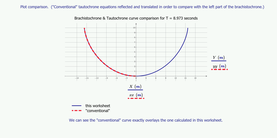
Editor's Note: Alan Stevens used the new plot formatting features available starting in PTC Mathcad Prime 12!

Extremely well done, Alan.

Larry Julyk’s Worksheet

Larry chose to derive the brachistochrone curve, which is no simple task. He starts with conservation of energy, Euler-Lagrange, and the Beltrami identity. His math regions and functions involve integrals, derivatives, prime operators, partial derivatives, and symbolic evaluation (similar to Alan’s worksheet).

He solves for x and y in terms of the angle theta, then applies boundary conditions to find a governing equality between x, y, and the angle. He uses a Solve Block to find the angle, which results in parametric equations that match the equation for a cycloid.

Larry takes this information to derive the equation for the travel time of the brachistochrone. For comparison, he derives the travel time for a straight line path between the two points. He graphs both paths on an XY plot. The brachistochrone certainly looks longer. However, given the initial conditions of an example, the brachistochrone takes approximately 2.3 seconds, whereas the straight line path takes 5.4 seconds! That’s considerably more than twice as long!

A second XY plot depicts the velocity of the object as a function of horizontal position for the brachistochrone and the straight line path. We can see why there is such a disparity in travel time: the brachistochrone quickly builds to a much higher velocity, where it stays throughout the journey until the end. (It makes sense that both paths result in the same final velocity, given that the initial potential energy is converted to the final kinetic energy.)

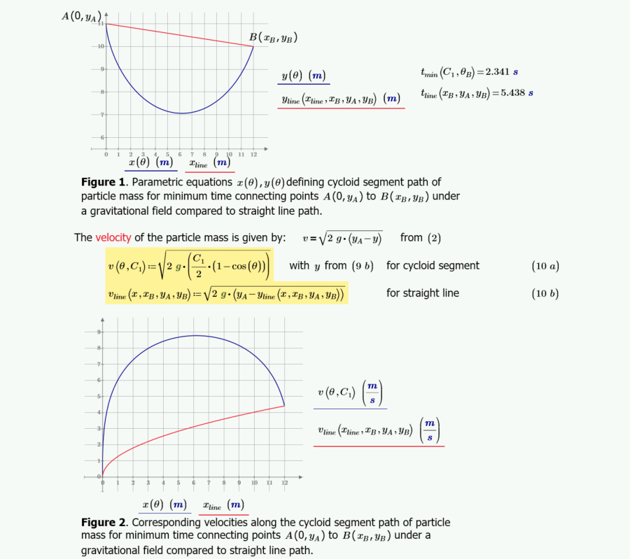
Larry created quite the worksheet. It derives the brachistochrone, shows that it is a cycloid, and then gives an example that demonstrates why it’s so much faster than the shortest path.

What can we learn?

This month’s challenge shows it’s truly not quantity that matters, but quality. We have two great worksheets that can stand on their own as teaching tools. The problem of tautochrone and brachistochrone curves are essentially physics problems, but these worksheets show that these are excellent teaching tools for students of calculus, given the wide variety of mathematical tools that Alan and Larry employ.

If you have an interest in learning physics and math, check out these excellent worksheets.